 The image at right shows the plate current pulse for a conduction angle
over 180 degrees.
The image at right shows the plate current pulse for a conduction angle
over 180 degrees.
GO TO Home Page
for more technical articles.
The last thirty years of my work experience involved the maintenance of high power AM television transmitters and related equipment. Some of these transmitters were capable of a RF power output of 35,000 watts at peak sinc levels in the AM TV bands near 200 Mhz.
.
There are a few reasons one might want to know the operating parameters
of the commonly used class AB power amplifiers:
Adjustment of loading on the plate circuit for most efficient operation,
Adjustment of plate voltage for most efficient operation,
Estimate the linearity and accuracy of in-line wattmeters,
and calculate resonant load resistance to calculate tank circuit 'Q',
and judge alignment of double tuned plate tanks.
Calculate the harmonic content which must be suppressed by the tank circuit.
.
I am assuming the reader has some technical knowledge of RF Amplifiers. The class AB amplifier has a conduction angle of greater than 180 degrees but less than 360 degrees. In practice, the conduction angle of plate current pulses are usually between 185 degrees and 200 degrees at maximum power output. Assume stiff power supplies for, plate, screen grid, and bias.
The theory behind the calculations is fairly simple.
First, find the conduction angle of the plate current pulse. This is done
graphically because the integral for analyzing the plate current pulse can
not be worked backwards by any mathematical formulas. We can integrate
the plate current pulse for trial values of conduction angle and plot
the results on a graph. We know the idle current of the amplifier and
the average plate current during operation. The conduction angle is
read off the graph opposite the ratio of plate current to idle current.
The peak value of the plate current pulse can be calculated from the
conduction angle.
Secondly, use Fourier's integral to analyze the plate current pulse for fundamental frequency content, along with the lower harmonics. Formulas can be used to calculate Fourier coefficients, once conduction angle is known. Trial values of conduction angle can also be used here to produce a graph of the Fourier coefficients for the fundamental frequency and lower harmonics. The Fourier fundamental frequency coefficient for a given conduction angle is multiplied by the peak value of the plate current pulse to find the fundamental RF frequency current contained in that conduction angle. Once one has the fundamental RF current, the fundamental RF voltage and resonant load resistance can be calculated from the amplifier power output.
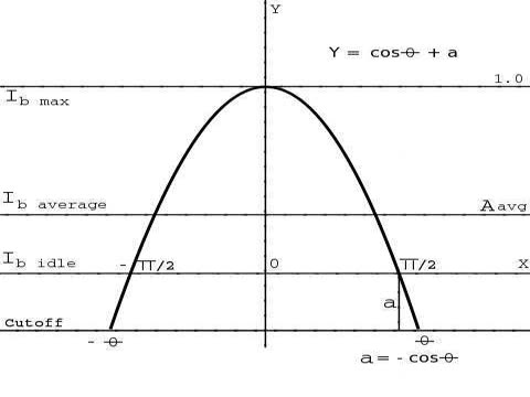
The image at right shows the plate current pulse for a conduction angle
over 180 degrees.
Integration to find the area under the curve can be simplified by using a
cosine wave, which is symmetrical about the zero 'Y' axis, and multiplying
the result by 2. That gives us the area under the curve and dividing by 2
Π gives the area average for the full 360 degree cycle.
Note:
that Θ equals the conduction angle divided by 2, as we are using the
cosine wave. Also note that radian measure is used!
On the left, Iidle, and Ib, which is the plate current with a black picture (no setup). On the right, are the values in trigonometry. The idle current 'a' equals ' -(cos Θ)'. Note that (cos Θ) is negative and -(cos Θ) results in a positive value. The plate current pulse is described by: y = (cos Θ + a) and the integral is ∫ (cos Θ + a). This is a simple integration from a book of integrals. Integration yields: A = (sin Θ + aΘ) and dividing by 2Π yields: Aavg = 1/Π (sin Θ + aΘ) for the complete 360 degree cycle.
Inspection of the plate current pulse gives us some proportions:
Ib / Iidle = Aavg / - cosΘ,
Ib max / Iidle = (1 - cosΘ) / - cosΘ, and
Ib max / Ib = (1 - cosΘ) / Aavg
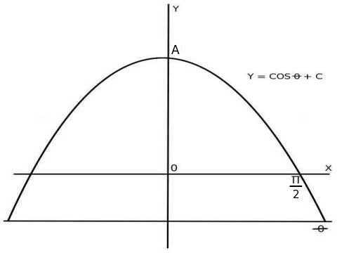 As above, the image at right shows the plate current pulse for a conduction
angle over 180 degrees. Again, we shall use the cosine function for ease
in integration, and multiply the result by 2. Again, Θ equals the
conduction angle divided by 2.
As above, the image at right shows the plate current pulse for a conduction
angle over 180 degrees. Again, we shall use the cosine function for ease
in integration, and multiply the result by 2. Again, Θ equals the
conduction angle divided by 2.
'N' below is the number of the harmonic content contained in the cosine wave. N = 1, is the fundamental component and N = 2, is the second harmonic, etc.
an = 2/Π∫ f(Θ) cos NΘ
dΘ, and from the integral sign to the right
we have
∫ (cosΘ = a) cos NΘ dΘ =
∫ u dv = uv - ∫ v du
where u = cos (Θ + a), dv = cos NΘ, du = - sin Θ,
and v = ∫ cos NΘ = (sin NΘ) / N
After integration, the formula for the fundamental Fourier coefficient is:
a1 = 2/Π [Θ/2 - (sin 2Θ)/4],
and the harmonic coefficients can be found by:
an = 2/Π N [sin(1-N)Θ / 2(1-N) - sin(1-N)Θ / 2(1+N)]
The peak value of the fundamental RF component of the plate current pulse is
i1, and
i1 = a1 B / (1 - cos Θ), where 'B' is the peak
value of the plate current pulse, I b max, and Ib
max = Iidle(1 - cosΘ) / - cosΘ
Combining the above two formulas and simplifying yields:
i1 = a1 Iidle / - cosΘ
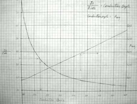 Back in the day - before computers - one would make a graph of conduction
angle vs Aavg and the ratio of Ib / Iidle.
The image to the right is an example.
Back in the day - before computers - one would make a graph of conduction
angle vs Aavg and the ratio of Ib / Iidle.
The image to the right is an example.
Ib is read from the
transmitter plate current meter. Ib / Iidle is on
the left side of the graph and the conduction angle is at the bottom. The
curved line is the locus of those points. On the right side of the graph
is Aavg and the locus of those points is the straight line.
Using a computer program, one can evaluate the expressions:
Aavg = 1/Π (sin Θ + aΘ),
Ib / Iidle = Aavg / - cosΘ,
a1 = 2/Π [Θ/2 - (sin 2Θ)/4], and
i1 = a1 Iidle / - cosΘ
in increments of 0.05 degrees from 185 degrees to 270 degrees and print the results to a table in a text file. Remember to convert degrees into radians for these formulas.
It is not even necessary to make a graph of these two functions. Average
plate current is read from the transmitter plate current ammeter and the
ratio of Ib / Iidle can be read directly from the
table in the text file. For example, an average plate current of 3.80
amperes and an idle current of 0.8 amperes yields an Ib /
Iidle of 4.7500. The closest Ib / Iidle
in the chart excerpt below is 4.757275 in the third line and the conduction
angle is 188.60 degrees and Aavg is 0.356694.
Ib/Iidle 4.806988, CA 188.50, A-avg 0.356239, a1 0.547136, i1 7.382902
Ib/Iidle 4.781985, CA 188.55, A-avg 0.356466, a1 0.547412, i1 7.343512
Ib/Iidle 4.757275, CA 188.60, A-avg 0.356694, a1 0.547688, i1 7.304581
Ib/Iidle 4.732851, CA 188.65, A-avg 0.356922, a1 0.547964, i1 7.266100
Ib/Iidle 4.708709, CA 188.70, A-avg 0.357150, a1 0.548241, i1 7.228062
The column 'a1' is the Fourier coefficient for the conduction angle and the
column 'i1' is the fundamental current component contained in the plate
current pulse.
Note: The column 'i1' is for an Iidle of '1' or unity.
This 'i1' must be normalized to a different Iidle by multiplying
this number by the different Iidle.
Note that milliamperes works just as well for Iidle and
Ib but do not mix milliamperes and amperes. If you start out
with one unit of measure, use them for all calculations!
If one knows Ib, Iidle, and the conduction angle, the other important parameters needed to start calculations are: plate voltage, Eb; screen grid voltage, Eg2; and the average amplifier output power, Po amp.
Note: If anyone wants the complete table above, send an E-Mail to the address at the end of this page and I will send the table as an attachment to an E-Mail back to you.
Formula one: Power delivered by the plate circuit, Pplate = P o amp / Ncir, where Po amp is the amplifier output power delivered to a load, and Ncir is the efficiency factor for the plate tank circuit.
Formula two: Peak voltage of plate circuit RF, e1 = 2 Pplate / i1, where i1 is the fundamental RF current component of the plate current pulse.
Formula three: Resonant load resistance, RL = e1 / i1
Formula four: Plate voltage efficiency factor, Ne = e1 / Eb, where Eb is the plate DC voltage.
Formula five: Conduction angle efficiency factor, NΘ = a1 / 2 Aavg, where a1 is the Fourier coefficient from tables as is Aavg.
Formula six: Amplifier efficiency factor, Namp = Ne NΘ Ncir
Formula seven: Also, amplifier efficiency factor, Namp = Po amp / Eb Ib, where Eb and Ib are the DC plate voltage and average current respectively.
Formula eight: Power, plate dissipation, Pp = (1 - Np) Eb Ib, where Np = plate circuit efficiency factor, Ne NΘ.
Formula nine: 'Q' or 'quality factor' = RL / Xc out, where Xc out is the reactance of the output capacitance of the tube, from the tube data sheet.
Formula ten: peak RF voltage at peak sinc, epk sinc = e2 = 2 Pplate pk sinc RL, where Pplate pk sinc is the power delivered by the plate circuit at peak sinc levels, or Pplate * 1.68.
Formula eleven: Eb min = Eb - epk sinc
Formula twelve: Voltage amplification factor, Av = e1 / e1 in, where e1 in is the drive voltage input to the cathode.
Formula thirteen: Current amplification factor, Ai = i1 / i1 in, where i1 in is the drive current input to the cathode.
Formula fourteen: Cathode input resistance, Rin = e1 in / i1, - or - in the case of the grounded grid amplifier, Rin = RL / Av.
Formula fifteen: Power gain, Gp = Av 2 Rin / RL, - or - Ai 2 RL / R in, - or - in the case of the grounded grid amplifier, Av, - or - RL / Rin.
The example television transmitter is a General Electric TT-B510 and B530 final visual RF amplifier combination. The B530 amplifier runs a pair of 4CX15000 tetrode tubes. These tubes are feed 90 degrees out of phase through a hybrid splitter and the two amplifier outputs are combined by a hybrid combiner. This hybrid combiner sums the RF back in-phase for feeding the transmission line to a second hybrid combiner. This second hybrid combiner sums the outputs of the visual and aural final amplifiers together and splits the combined output into two components which are 90 degrees out of phase. One output feeds the transmission line to the antenna for the North-South direction, and the other output feeds the transmission line to the antenna for the East-West direction.
The 4CX15000 RF amplifiers are of the grounded grid configuration where both the control and screen grids are grounded for RF and the tube is fed via cathode. The plate is also grounded for RF, for those who are familiar with TE mode aperture coupling where the electron stream within the tube is coupled to the tank cavity through the ceramic section of the tube. The standard grounded grid circuit model is used for calculations. The plate tank is a double tuned circuit. The primary circuit is a cavity which contains the amplifier tube, and the secondary circuit is a coupling link to the primary, with series and shunt air variable tuning capacitors. The bandwidth of the tank circuit is approximately 4.2 Mhz. The efficiency factor, Ncir is estimated to be 0.9 for this tank circuit and 0.95 for the input matching circuit feeding the amplifier.
Typical operation:
Frequency of operation: channel 13, with visual carrier at 211.125 Mhz.
Total power output = 30,000 watts at peak sinc levels.
Plate voltage, Eb = 6000 volts DC.
Plate current, Ib = 3.80 amperes average at black picture for
each tube.
Plate current at idle, Iidle = 0.8 amperes.
Screen grid voltage, Eg2 = 750 volts DC.
Screen grid current, Ig2 = 100 milliamperes DC.
Each amplifier delivers 15,000 watts at peak sinc level.
The wattmeter measures average transmitter power with a black picture, and
the ratio of peak sinc to average level is 1.68 - so Po amp = 8929
watts average with a black picture.
Formula one: Power delivered by the plate circuit, Pplate = Po amp / Ncir, where Po amp is the amplifier output power delivered to a load, and Ncir is the efficiency factor for the plate tank circuit. Pplate = 8929 / 0.9 = 9921 watts.
From the table excerpt above:
Ib / Iidle = 4.7500 and
the conduction angle = 188.6 degrees and i1 = 7.304581 amperes
peak which is the value for an Iidle of 1 ampere. In this case,
7.304581 * 0.8 = 5.844 amps, which is the peak value of the fundamental RF
current component of the plate current pulse.
Formula two: Peak voltage of plate circuit RF, e1 = 2 Pplate / i1, where i1 is the fundamental RF current component of the plate current pulse. e1 = 2 * 9921 / 5.844 = 3396 volts peak of fundamental RF component.
Formula three: Resonant load resistance, RL = e1 / i1 = 3396 / 5.844 = 581 ohms.
Formula four: Plate voltage efficiency factor, Ne = e1 / Eb, where Eb is the plate DC voltage. Ne = 3396 / 6000 = 0.5660
Formula five: Conduction angle efficiency factor, NΘ
= a1 / 2 Aavg, from the table excerpt above, and
0.547688 / 2 * 0.356694 = NΘ = 0.7677
Formula six: Amplifier efficiency factor, Namp =
Ne NΘ Ncir, and
0.5660 * 0.7677 * 0.9 = 39.11 percent.
Formula seven: Also, amplifier efficiency factor, Namp =
Po amp / Eb Ib, and
8929 / 6000 * 3.80 = 39.16 percent.
The results of Formula six and Formula seven are very close together in value. This is the acid test of the accuracy of the integration of the plate current pulse, the solution to Fourier's integral, and the calculations up to this point.
Formula eight: Power, plate dissipation, Pp = (1 -
Np) Eb Ib, where Np =
plate circuit efficiency factor, Ne NΘ, and
(1 - 0.5660 * 0.7677) * 6000 * 3.80 = 12,893 watts, which is below the
maximum of 15,000 watts plate dissipation for the 4CX15000 tube.
Formula nine: 'Q' or 'quality factor' = RL / Xc
out, where Xc out is the reactance of the output
capacitance of the tube, where 'c out' = 24.5 pf, from the tube data sheet
and 'Q' = 581 / 30.769 = 18.88.
The maximum allowable 'Q' is probably around 20. A higher operating 'Q'
results in higher circulating currents in the double tuned tank circuit
causing excessive heating and possible destruction, as witnessed in a few
cases.
Formula ten: peak RF voltage at peak sinc, epk sinc = e2 = 2 Pplate pk sinc RL, and (2 * 9921 * 1.68 * 581)1/2 = 4401 volts at peak sinc level.
Formula eleven: Eb min = Eb - epk
sinc, and 6000 - 4401 = 1599 volts. This is the absolute value of
the negative excursion of the RF at peak sinc levels. If the RF voltage
swing becomes greater, this value approaches Eg2 = 750 volts,
and Ig2 increases. If Ig2 increases substantially
above the 100 ma of ty#928cal operation, the amplifier becomes non-linear.
This condition may also indicate error in the alignment of the double tuned
tank circuit. A double humped swept frequency response, which has higher
amplitude at the visual carrier frequency, will have higher than normal
resonant load resistance, RL.
It is the RF voltage at peak sinc modulation levels which limit the
amplifier efficiency at average power.
Formula twelve: Voltage amplification factor, Av =
e1 / e1 in, where e1 in is the drive
voltage input to the cathode. From the tube data sheet, approximate drive
voltage is 345 volts at peak sinc, or 266 volts at average power, and
the voltage amplification factor is 3396 / 266 = 12.767
Formula thirteen: Current amplification factor, Ai =
i1 / i1 in, where i1 in is the drive
current input to the cathode.
The grounded grid amplifier has a current amplification factor of 1 (one).
Formula fourteen: Cathode input resistance, Rin =
e1 in / i1, or in the case of the grounded grid
amplifier, Rin = RL / Av.
266 / 5.844 = 45.57 ohms, - or - 581 / 12.767 = 45.51 ohms approximate cathode
input resistance. This is close to the nominal 50 ohm impedance of
transmission line and a simple low 'Q' broadband Π or T network will
suffice for matching to the preceding driver amplifier.
Formula fifteen: Power gain, Gp = Av
2 Rin / RL, - or - Ai 2
RL / R in, - or - in the case of the grounded grid
amplifier, Av, - or - RL / Rin.
In the case of the grounded grid amplifier, Gp = Av,
or 12.767 approximately.
This example calculates the operating parameters for a different power output from the same amplifier.
From above, the average power delivered by the plate circuit, Pplate is 9921 watts with a black picture at 100 percent power and, RL is 581 ohms.
What are the amplifier operating parameters at 50 percent power?
9921 * 0.5 = 4960.5 watts delivered by the plate circuit.
i12 = 2 Pplate / RL, and
(2 * 4960.5 / 581)1/2 = i1 = 4.1323 amperes.
Note: this is at an Iidle of 0.8 amperes DC. Divide the
i1 by 0.8 amperes to get the i1 at an idle current of
1.0 amperes: 4.1323 / 0.8 = i1 = 5.1653
The 5.1653 figure is only for use with the computer generated tables.
i1 = 4.1323 amperes for 50 percent amplifier power output.
From the computer generated tables, the closest i1 is 5.156047 in the middle line below in the far right column. Also, conduction angle = 192.70 degrees, Ib / Iidle = 3.395605. Since Iidle = 0.8, Ib = 2.716 amperes DC.
Ib/Iidle 3.418215, CA 192.60, A-avg 0.375095, a1 0.569719, i1 5.191800
Ib/Iidle 3.406865, CA 192.65, A-avg 0.375328, a1 0.569993, i1 5.173853
Ib/Iidle 3.395605, CA 192.70, A-avg 0.375560, a1 0.570267, i1 5.156047
Ib/Iidle 3.384435, CA 192.75, A-avg 0.375792, a1 0.570542, i1 5.138381
Ib/Iidle 3.373352, CA 192.80, A-avg 0.376024, a1 0.570816, i1 5.120854
Formula ten: peak RF voltage, e1 = e2 = 2 Pplate RL, and (2 * 4960.5 * 581)1/2 = e1 =2401 volts.
Formula four: Plate voltage efficiency factor, Ne = 2401 / 6000 = Ne = 0.40012
Formula five: Conduction angle efficiency factor, NΘ
= a1 / 2 Aavg, from the table excerpt above, and
0.570267 / 2 * 0.375560 = NΘ = 0.75921
Formula six: Amplifier efficiency factor, Namp =
Ne NΘ Ncir, and
0.40012 * 0.75921 * 0.9 = 27.34 percent.
Formula seven: Also, amplifier efficiency factor, Namp =
Po amp / Eb Ib, where Po amp =
Pplate Ncir, and
4960.5 * 0.9 / 6000 * 2.716 = 27.40 percent which compares well with the
27.34 percent above.
Formula eight: Power, plate dissipation, Pp = (1 -
Np) Eb Ib, where Np = plate
circuit efficiency factor, Ne NΘ, and
(1 -
0.40012 * 0.75921) * 6000 * 2.716 = Pp = 11,346 watts plate
dissipation.
Note: At 100 percent power, Pp = 12,893 watts. Reducing the
output power by 50 percent only reduced the plate dissipation by 12
percent.
.
The engineer in charge of maintenance on the above television transmitter told me that he was getting an efficiency of 55 percent. I asked if he thought that might be a red flag as I knew that was not possible. He said that class AB amplifiers were capable of that efficiency. It took some convincing but I finally got him to borrow a different thru-line wattmeter from one of our other transmitter sites. I heard later that when he tried to do a transmitter power meter calibration with the borrowed wattmeter, the screen grid current, Ig2, became very high at only 50 percent of licensed power and sinc pulses were very compressed and the chroma levels were quite low, which were signs of a badly mistuned plate tank circuit. The transmitter had only ran another day when the secondary tuning sections of both of the plate tank circuits had burned up.
This transmitter had a built in sweep generator and diode detectors on the amplifier output for use in alignment, which was done at zero power with no DC plate voltage applied. The engineer had been doing the alignment like on our other transmitters, by applying video sweep into the visual modulator and connecting a spectrum analyzer to directional couplers in the transmission lines at the amplifier outputs. The diode detectors are not directional couplers, and the limiting action of the diodes made the frequency response of the plate tank circuit look good even though it was peaked up high over the visual carrier frequency. The resulting high resonant load resistance, RL, and much higher circuit 'Q', caused the secondary sections of both tank circuits to overheat.
The example amplifiers above use the grounded grid configuration but the calculations involving the plate circuit are the same for the grounded cathode circuit as well. The difference in formulas is related to the amplifier input, and are included in the formula section above in Formulas Thirteen, Fourteen, and Fifteen.
The frequency of operation will have an effect on the estimated value of the tuned circuit efficiency factor, Ncir, for the plate tank circuit and the matching network to the amplifier inputs. The estimate of Ncir = 0.9 for the plate tank circuit, and 0.95 for the input matching network is for a frequency of around 200 Mhz. and comes from the transmitter manufacturer. Higher operating frequencies will cause less efficiencies and lower operating frequencies will cause higher efficiencies. How much lower or higher? Use your best guess, unless someone actually knows. In the HF range, the heating loss in those circuits is probably only a few percent and the error in the estimate should not cause significant error in the calculated results.
Inaccurate wattmeters are the most common source of error. An accurate power measurement is essential! A careful power measurement using a calorimeter is preferred.
Note that Formulas nine and twelve require values from the tube data sheet.
Linear Amplifiers for Single Sideband
The amplifier must be operated within its linear limits. If the amplifier input is fed with RF modulated with steady state two tone audio, the plate current ammeter will read the average plate current, Ib. Read the ratio of Ib / Iidle in the tables (or graph) to find conduction angle, Aavg, a1, and i1. Multiply i1 by the Iidle current and proceed with calculations starting with Formula one.
The ratio of the power at the peak of the modulation envelope to average power is a factor of 2.0. When you get to Formula ten, substitute 2.0 in place of the 1.68 used for video, to find e1 at the peak of the modulation envelope.
Linear Amplifiers for FM
Again, the amplifier must be operated within its linear limits. There is no amplitude modulation envelope, so average power output and peak power output are the same! Read across from Ib / Iidle in the tables, multiply i1 by the Iidle current and proceed with calculations starting with Formula one. Skip Formula ten, and use e1 in Formula eleven.
Comments on the Calculations
* You get to Formula eleven and find that Eb min is less than Eg2 and Ig2 is not excessive, or in the case of a triode tube or transistor, that Eb min is less than zero, and there is no distortion on the amplifier output.
Wattmeters seem to err on the safe side. This is an indication that the amplifier output is somewhat lower than the wattmeter indicates. Calculations result in a resonant load resistance which is falsely too high, and swing of e1 which is falsely too high.
* How accurate and how linear is your in-line or other wattmeter?
Take wattmeter, Po amp, and amplifier meter readings, Ib, at 25, 50, 75, and 100 percent power and do the calculations for each as far as Formula three for resonant load resistance, RL. The resonant load resistance should calculate to nearly the same in each case, allowing for a couple percent error for meter reading error. If the resonant load resistance steadily increases or steadily decreases, the wattmeter is non-linear for power, and any readings from it are suspect.
* What is the harmonic power which must be suppressed by the tank circuit?
Calculate an = 2/Π N [sin(1-N)Θ / 2(1-N) - sin(1-N)Θ
/ 2(1+N)], for your conduction angle at average power. 'N' is the number
of the harmonic: N=2 is second harmonic, N=3 is third, etc.
Plug the an into the formula: in = an
Iidle / - cosΘ, to find the amplitude of the harmonic
current, and the power is: in2 RL / 2.
Remember, Θ is conduction angle / 2, and use radian measure in the
above formulas!
This article was written using notes I made while doing research back in the late 1980s and early 1990s. I did not keep track of the references. Some of the formulas came from a 1950s McGraw-Hill 'Radio Handbook' and some were derived by me.
I was on my own for the sections on integrating the plate current pulse, and the related proportions, and the solution to Fourier's integral. It was not treated in enough depth in college, and I could find almost nothing with enough depth in our local libraries, or in my own reference collection. It took me a while to get it right! I am sure others before me have done this. I was just not lucky enough to discover their work.
.